DDPM Explanation by Bayes’ Perspective
In the following session, we will discuss the DDPM forward and backward pass via Bayes’ Theorem. It help the speed up introduced in DDIM.
Recall of Completing the Square
We have a quadratic form as follows:
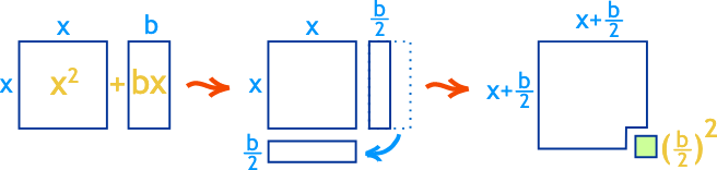
By formulas, we have \(\begin{gather} \therefore d = \frac{b}{2a} \\ e = c - \frac{b^2}{4a} = c - d^2 \end{gather}\)
Recall of Bayes’ Theorem
Bayes' theorem is defined as follows:
\[\begin{equation}p(\boldsymbol{x}_{t-1}|\boldsymbol{x}_t) = \frac{p(\boldsymbol{x}_t|\boldsymbol{x}_{t-1})p(\boldsymbol{x}_{t-1})}{p(\boldsymbol{x}_t)}\end{equation}\]However, we do not know the expression formulas of $p(\boldsymbol{x}_{t-1}),p(\boldsymbol{x}_t)$. Luckily, we can add one more condition$\boldsymbol{x}_0$ s.t.
\[\begin{aligned} p(\boldsymbol{x}_{t-1}|\boldsymbol{x}_t, \boldsymbol{x}_0) &= \frac{p(\boldsymbol{x}_{t-1},\boldsymbol{x}_t, \boldsymbol{x}_0)}{p(\boldsymbol{x}_t, \boldsymbol{x}_0)}\\ &= \frac{p(\boldsymbol{x}_{t}|\boldsymbol{x}_{t-1}, \boldsymbol{x}_0)p(\boldsymbol{x}_{t-1}, \boldsymbol{x}_0)}{p(\boldsymbol{x}_t| \boldsymbol{x}_0)p(\boldsymbol{x}_0)}\\ &= \frac{p(\boldsymbol{x}_{t}|\boldsymbol{x}_{t-1}, \boldsymbol{x}_0)p(\boldsymbol{x}_{t-1}| \boldsymbol{x}_0)\cancel{p(\boldsymbol{x}_0)}}{p(\boldsymbol{x}_t| \boldsymbol{x}_0)\cancel{p(\boldsymbol{x}_0)}}\\ \end{aligned}\]Therefore, in diffusion model,
\[\begin{equation} p(\boldsymbol{x}_{t-1}|\boldsymbol{x}_t, \boldsymbol{x}_0)= \frac{p(\boldsymbol{x}_t|\boldsymbol{x}_{t-1})p(\boldsymbol{x}_{t-1}|\boldsymbol{x}_0)}{p(\boldsymbol{x}_t|\boldsymbol{x}_0)} \end{equation}\]where \(p(\boldsymbol{x}_t\vert\boldsymbol{x}_{t-1}),p(\boldsymbol{x}_{t-1}\vert\boldsymbol{x}_0),p(\boldsymbol{x}_t\vert\boldsymbol{x}_0)\) is well known or can be found.
Therefore, we can get the following expression:
\[\begin{aligned} p(\boldsymbol{x}_t|\boldsymbol{x}_{t-1}) &= \boldsymbol{N}(\boldsymbol{x}_t; \sqrt{\alpha_t}\boldsymbol{x}_{t-1};\beta_t\boldsymbol{I}) \\ p(\boldsymbol{x}_{t-1} \vert \boldsymbol{x}_0) &= \boldsymbol{N}(\boldsymbol{x}_{t-1}; \sqrt{\bar{\alpha}_{t-1}} \boldsymbol{x}_0, (1-\bar{\alpha}_{t-1})\boldsymbol{I}) \\ p(\boldsymbol{x}_t \vert \boldsymbol{x}_0) &= \boldsymbol{N}(\boldsymbol{x}_t; \sqrt{\bar{\alpha}_t} \boldsymbol{x}_0, (1-\bar{\alpha_t})\boldsymbol{I}) \end{aligned}\]We put all expression above to compute:
\[\begin{aligned} p(\mathbf{x}_{t-1} \vert \mathbf{x}_t, \mathbf{x}_0) &= p(\mathbf{x}_t \vert \mathbf{x}_{t-1}, \mathbf{x}_0) \frac{ p(\mathbf{x}_{t-1} \vert \mathbf{x}_0) }{ p(\mathbf{x}_t \vert \mathbf{x}_0) } \\ &\propto \exp \Big(-\frac{1}{2} \big(\frac{(\mathbf{x}_t - \sqrt{\alpha_t} \mathbf{x}_{t-1})^2}{\beta_t} + \frac{(\mathbf{x}_{t-1} - \sqrt{\bar{\alpha}_{t-1}} \mathbf{x}_0)^2}{1-\bar{\alpha}_{t-1}} - \frac{(\mathbf{x}_t - \sqrt{\bar{\alpha}_t} \mathbf{x}_0)^2}{1-\bar{\alpha}_t} \big) \Big) \\ &= \exp \Big(-\frac{1}{2} \big(\frac{\mathbf{x}_t^2 - 2\sqrt{\alpha_t} \mathbf{x}_t \color{blue}{\mathbf{x}_{t-1}} \color{black}{+ \alpha_t} \color{red}{\mathbf{x}_{t-1}^2} }{\beta_t} + \frac{ \color{red}{\mathbf{x}_{t-1}^2} \color{black}{- 2 \sqrt{\bar{\alpha}_{t-1}} \mathbf{x}_0} \color{blue}{\mathbf{x}_{t-1}} \color{black}{+ \bar{\alpha}_{t-1} \mathbf{x}_0^2} }{1-\bar{\alpha}_{t-1}} - \frac{(\mathbf{x}_t - \sqrt{\bar{\alpha}_t} \mathbf{x}_0)^2}{1-\bar{\alpha}_t} \big) \Big) \\ &= \exp\Big( -\frac{1}{2} \big( \color{red}{(\frac{\alpha_t}{\beta_t} + \frac{1}{1 - \bar{\alpha}_{t-1}})} \mathbf{x}_{t-1}^2 - \color{blue}{(\frac{2\sqrt{\alpha_t}}{\beta_t} \mathbf{x}_t + \frac{2\sqrt{\bar{\alpha}_{t-1}}}{1 - \bar{\alpha}_{t-1}} \mathbf{x}_0)} \mathbf{x}_{t-1} \color{black}{ + C(\mathbf{x}_t, \mathbf{x}_0) \big) \Big)} \\ &= \exp\Big( -\frac{1}{2} \big( \color{red}{(\frac{\alpha_t}{\beta_t} + \frac{1}{1 - \bar{\alpha}_{t-1}})} \mathbf{x}_{t-1}^2 - \color{blue}{(\frac{2\sqrt{\alpha_t}}{\beta_t} \mathbf{x}_t + \frac{2\sqrt{\bar{\alpha}_{t-1}}}{1 - \bar{\alpha}_{t-1}} \mathbf{x}_0)} \mathbf{x}_{t-1} \color{black}{ + C(\mathbf{x}_t, \mathbf{x}_0) \big) \Big)} \\ &= \exp\Big( -\frac{1}{2} \big( \color{red}{(\frac{\alpha_t}{\beta_t} + \frac{1}{(1-\bar{\alpha}_{t-1})})} \mathbf{x}_{t-1}^2 - \color{blue}{(\frac{2\sqrt{\alpha_t}}{\beta_t} \mathbf{x}_t + \frac{2\sqrt{\bar{\alpha}_{t-1}}}{(1-\bar{\alpha}_{t-1})} \mathbf{x}_0)} \mathbf{x}_{t-1} \color{black}{ + C(\mathbf{x}_t, \mathbf{x}_0) \big) \Big)} \\ &= exp\Big(-\frac{1}{2}\big(\color{red}{a}\color{black}{(x+}\color{blue}{d})^2 \color{black}{+ e} \big)\Big) \\ &= \boldsymbol{N}( d , \frac{1}{a}\boldsymbol{I}) \end{aligned}\]Recall that $f(x)=\frac{1}{\sqrt{2 \pi} \sigma_f} exp\Big({-\frac{1}{2}\frac{\left(x-\color{blue}{\mu_f}\right)^2}{\color{red}{\sigma_f^2}}}\Big) = \boldsymbol{N}(\mu_f, \sigma^2_f)$
We can focus on getting the coefficient of $\boldsymbol{x}_{t-1}^2$. As this term is quadratic, this implies the final format also follow gaussian distribution. We get the quadratic form by completing the square:
\[\begin{aligned} a = \frac{\alpha_t}{\beta_t} + \frac{1}{(1-\bar{\alpha}_{t-1})} = \frac{\alpha_t(1-\bar{\alpha}_{t-1}) + \beta_t}{(1-\bar{\alpha}_{t-1}) \beta_t} &= \frac{\alpha_t(1-\bar{\alpha}_{t-1}) + \beta_t}{(1-\bar{\alpha}_{t-1}) \beta_t} = \frac{1-\bar{\alpha}_t}{(1-\bar{\alpha}_{t-1}) \beta_t} = \frac{(1-\bar{\alpha_t})}{(1-\bar{\alpha}_{t-1}) \beta_t} \\ \therefore p(\mathbf{x}_{t-1} \vert \mathbf{x}_t, \mathbf{x}_0) &= \boldsymbol{N}( d , \frac{(1-\bar{\alpha}_{t-1}) \beta_t}{(1-\bar{\alpha_t})}\boldsymbol{I} ) \end{aligned}\]Therefore,
\[\begin{aligned} d = \frac{b}{2a} &= (\frac{\sqrt{\alpha_t}}{\beta_t} \mathbf{x}_t + \frac{\sqrt{\bar{\alpha}_{t-1} }}{1 - \bar{\alpha}_{t-1}} \mathbf{x}_0)/(\frac{\alpha_t}{\beta_t} + \frac{1}{1 - \bar{\alpha}_{t-1}}) \\ &= (\frac{\sqrt{\alpha_t}}{\beta_t} \mathbf{x}_t + \frac{\sqrt{\bar{\alpha}_{t-1} }}{1 - \bar{\alpha}_{t-1}} \mathbf{x}_0) \color{green}{\frac{1 - \bar{\alpha}_{t-1}}{1 - \bar{\alpha}_t} \cdot \beta_t} \\ &= \frac{\sqrt{\alpha_t}(1 - \bar{\alpha}_{t-1})}{1 - \bar{\alpha}_t} \mathbf{x}_t + \frac{\sqrt{\bar{\alpha}_{t-1}}\beta_t}{1 - \bar{\alpha}_t} \mathbf{x}_0\\ &= \frac{\sqrt{\alpha_t}(1-\bar{\alpha}_{t-1})}{(1-\bar{\alpha_t})}\boldsymbol{x}_t + \frac{\sqrt{\bar{\alpha}_{t-1}}\beta_t}{(1-\bar{\alpha_t})}\boldsymbol{x}_0 \\ \end{aligned}\]We can get the final distribution expression s.t.
\[\begin{equation} \therefore p(\boldsymbol{x}_{t-1}|\boldsymbol{x}_t, \boldsymbol{x}_0) = \mathcal{N}\left(\boldsymbol{x}_{t-1};\frac{\sqrt{\alpha_t}(1-\bar{\alpha}_{t-1})}{(1-\bar{\alpha_t})}\boldsymbol{x}_t + \frac{\sqrt{\bar{\alpha}_{t-1}}\beta_t}{(1-\bar{\alpha_t})}\boldsymbol{x}_0,\frac{(1-\bar{\alpha}_{t-1})\beta_t}{(1-\bar{\alpha_t})} \boldsymbol{I}\right) \end{equation}\]Revisit of denoising (reverse) process
We have $p(x_{t-1} \vert x_t, x_0)$, which has explicit expression from gaussian distribution. However, we cannot rely on getting $x_0$ to express such expression. $x_0$ should be our final output.
Therefore, we want to make the assumption as follows:
Can we use $x_t$ to predict $x_0$ s.t. we can escape the term of $x_0$ in $p(x_{t-1} \vert x_t, x_0)$ ?
With the model $\bar{u}(x_t) \text{ that predict } x_0 \text{ , where loss function }\boldsymbol{L} = \Vert x_0 - \bar{u}(x_t) \Vert^2$. This idea leads to the following expression:
\[\begin{equation} p(\boldsymbol{x}_{t-1}|\boldsymbol{x}_t) \approx p(\boldsymbol{x}_{t-1}|\boldsymbol{x}_t, \boldsymbol{x}_0=\bar{\boldsymbol{\mu}}(\boldsymbol{x}_t)) = \mathcal{N}\left(\boldsymbol{x}_{t-1}; \frac{\sqrt{\alpha_t}(1-\bar{\alpha}_{t-1})}{(1-\bar{\alpha_t})}\boldsymbol{x}_t + \frac{\sqrt{\bar{\alpha}_{t-1}}\beta_t}{(1-\bar{\alpha_t})}\bar{\boldsymbol{\mu}}(\boldsymbol{x}_t),\frac{(1-\bar{\alpha}_{t-1})\beta_t}{(1-\bar{\alpha_t})} \boldsymbol{I}\right) \end{equation}\]The word denoising in DDPM is coming from the loss function $ \Vert x_0 - \bar{u}(x_t) \Vert^2$ , where $x_0$ is the raw image (data) and $x_t$ refers to lossy image (data).
Recall \(\begin{aligned} p(\boldsymbol{x}_t \vert \boldsymbol{x}_0) &= \boldsymbol{N}(\boldsymbol{x}_t; \sqrt{\bar{\alpha}_t} \boldsymbol{x}_0, (1-\bar{\alpha_t})\boldsymbol{I}) \\ \boldsymbol{x}_t &= \sqrt{\bar{\alpha}_t} \boldsymbol{x}_0 + \sqrt{(1-\bar{\alpha_t})} \boldsymbol{\varepsilon},\boldsymbol{\varepsilon}\sim\mathcal{N}(\boldsymbol{0}, \boldsymbol{I}) \\ x_0 &= \frac{1}{\sqrt{\bar{\alpha_t}}}(x_t-\sqrt{\bar{\beta_t}}\boldsymbol{\epsilon)} \\ i.e. \space \bar{u}(x_t) &= \frac{1}{\sqrt{\bar{\alpha_t}}}\big(x_t-\sqrt{\bar{\beta_t}}\boldsymbol{\epsilon_\theta (x_t, t)}\big) \\ \boldsymbol{Loss} &= \frac{\beta_t}{\alpha_t}\left\Vert \boldsymbol{\varepsilon}_t - \boldsymbol{\epsilon}_{\boldsymbol{\theta}}(\sqrt{\bar{\alpha}_t}\mathbf{x}_0 + \sqrt{\bar{\beta}}\boldsymbol{\bar{\epsilon}}, t)\right\Vert^2 \end{aligned}\)
Insert $\bar{u}(t)$ into equation 6, we will get
\[\begin{aligned} p(\boldsymbol{x}_{t-1}|\boldsymbol{x}_t) \approx p(\boldsymbol{x}_{t-1}|\boldsymbol{x}_t, \boldsymbol{x}_0=\bar{\boldsymbol{\mu}}(\boldsymbol{x}_t)) &= \mathcal{N}\left(\boldsymbol{x}_{t-1}; \frac{\sqrt{\alpha_t}(1-\bar{\alpha}_{t-1})}{(1-\bar{\alpha_t})}\boldsymbol{x}_t + \frac{\sqrt{\bar{\alpha}_{t-1}}\beta_t}{(1-\bar{\alpha_t})}\Big( \frac{1}{\sqrt{\bar{\alpha_t}}}\big(x_t-\sqrt{\bar{\beta_t}}\boldsymbol{\epsilon_\theta (x_t, t)}\big) \Big),\frac{(1-\bar{\alpha}_{t-1})\beta_t}{(1-\bar{\alpha_t})} \boldsymbol{I}\right) \\ \frac{\sqrt{\alpha_t}(1-\bar{\alpha}_{t-1})}{(1-\bar{\alpha_t})}\boldsymbol{x}_t + \frac{\sqrt{\bar{\alpha}_{t-1}}\beta_t}{(1-\bar{\alpha_t})}\Big( \frac{1}{\sqrt{\bar{\alpha_t}}}\big(x_t-\sqrt{\bar{\beta_t}}\boldsymbol{\epsilon_\theta (x_t, t)}\big) \Big) &= \frac{\sqrt{\alpha_t}(1-\bar{\alpha}_{t-1})}{(1-\bar{\alpha_t})}\boldsymbol{x}_t + \frac{\sqrt{\bar{\alpha}_{t-1}}\beta_t}{(1-\bar{\alpha_t}) \sqrt{\bar{\alpha_t}}}\big(x_t-\sqrt{\bar{\beta_t}}\boldsymbol{\epsilon_\theta (x_t, t)}\big) \\ &= \Big(\frac{\sqrt{\alpha_t}(1-\bar{\alpha}_{t-1})}{(1-\bar{\alpha_t})} + \frac{\sqrt{\bar{\alpha}_{t-1}}\beta_t}{(1-\bar{\alpha_t}) \sqrt{\bar{\alpha_t}}} \Big)x_t - \frac{\sqrt{\bar{\alpha}_{t-1}}\beta_t}{(1-\bar{\alpha_t}) \sqrt{\bar{\alpha_t}}}\sqrt{\bar{\beta_t}}\boldsymbol{\epsilon_\theta (x_t, t)} \\ &= \frac{\sqrt{\bar{\alpha_t}}\sqrt{\alpha_t}(1-\bar{\alpha}_{t-1}) + \sqrt{\bar{\alpha}_{t-1}}\beta_t}{\sqrt{\bar{\alpha_t}}(1-\bar{\alpha_t})}x_t - \frac{\beta_t}{\sqrt{(1-\bar{\alpha_t})} \sqrt{\alpha_t}}\boldsymbol{\epsilon_\theta (x_t, t)} \\ &= \big(\frac{\alpha_t(1-\bar{\alpha_{t-1}}) + \beta_t}{\sqrt{\alpha_t}\bar{\beta_t}}\big)x_t - \frac{\beta_t}{\sqrt{(1-\bar{\alpha_t})} \sqrt{\alpha_t}}\boldsymbol{\epsilon_\theta (x_t, t)} \\ &= \big(\frac{(1-\beta_t)-\bar{\alpha_{t}} + \beta_t}{\sqrt{\alpha_t}\bar{\beta_t}}\big)x_t - \frac{\beta_t}{\sqrt{(1-\bar{\alpha_t})} \sqrt{\alpha_t}}\boldsymbol{\epsilon_\theta (x_t, t)} \\ &= \big(\frac{\bar{\beta_t}}{\sqrt{\alpha_t}\bar{\beta_t}}\big)x_t - \frac{\beta_t}{\sqrt{(1-\bar{\alpha_t})} \sqrt{\alpha_t}}\boldsymbol{\epsilon_\theta (x_t, t)} \\ &= \frac{1}{\sqrt{\alpha_t}}\big(x_t - \frac{\beta_t}{\sqrt{(1-\bar{\alpha_t})}}\boldsymbol{\epsilon_\theta (x_t, t)} \big) \end{aligned}\] \[\begin{equation} \therefore p(\boldsymbol{x}_{t-1}|\boldsymbol{x}_t) \approx p(\boldsymbol{x}_{t-1}|\boldsymbol{x}_t, \boldsymbol{x}_0 =\bar{\boldsymbol{\mu}}(\boldsymbol{x}_t)) = \mathcal{N}\left(\boldsymbol{x}_{t-1}; \frac{1}{\sqrt{\alpha_t}}\big(x_t - \frac{\beta_t}{\sqrt{(1-\bar{\alpha_t})}}\boldsymbol{\epsilon_\theta (x_t, t)} \big),\frac{(1-\bar{\alpha}_{t-1})\beta_t}{(1-\bar{\alpha_t})} \boldsymbol{I}\right) \end{equation}\]Conclusion
In short, we have discussed the derivation as follows: \(\begin{equation}p(\boldsymbol{x}_t|\boldsymbol{x}_{t-1})\xrightarrow{\text{derive}}p(\boldsymbol{x}_t|\boldsymbol{x}_0)\xrightarrow{\text{derive}}p(\boldsymbol{x}_{t-1}|\boldsymbol{x}_t, \boldsymbol{x}_0)\xrightarrow{\text{approx}}p(\boldsymbol{x}_{t-1}|\boldsymbol{x}_t)\end{equation}\)
We have found that
- Loss function is only related to $p(x_t\vert x_0)$
- Sampling process only rely on $p(x_{t-1} \vert x_t)$
Special Case in Variance Choice
As mentioned, we cannot apply \(p(\boldsymbol{x}_{t-1}\vert\boldsymbol{x}_t) = \frac{p(\boldsymbol{x}_t\vert\boldsymbol{x}_{t-1})p(\boldsymbol{x}_{t-1})}{p(\boldsymbol{x}_t)}\) directly as $p(x_{t-1})$ and \(p(\boldsymbol{x}_t) = \int p(\boldsymbol{x}_t|\boldsymbol{x}_0)\tilde{p}(\boldsymbol{x}_0)d\boldsymbol{x}_0\) is unknown, where we cannot get $\tilde{p}(\boldsymbol{x}_0)$ in advance, except:
Case 1: Only one sample in dataset
The dataset has only $\boldsymbol{0}$ and $\tilde{p}(\boldsymbol{x}_0) = \delta(\boldsymbol{x}_0)$ \(\begin{equation}p(\boldsymbol{x}_{t-1}|\boldsymbol{x}_t) = p(\boldsymbol{x}_{t-1}|\boldsymbol{x}_t, \boldsymbol{x}_0=\boldsymbol{0}) = \mathcal{N}\left(\boldsymbol{x}_{t-1};\frac{\sqrt{\alpha_t}(1-\bar{\alpha}_{t-1})}{(1-\bar{\alpha_t})}\boldsymbol{x}_t,\frac{(1-\bar{\alpha}_{t-1})\beta_t}{(1-\bar{\alpha_t})} \boldsymbol{I}\right)\end{equation}\)
We can get variance as $\frac{(1-\bar{\alpha}_{t-1})\beta_t}{(1-\bar{\alpha_t})}$. This is one of the choice on variance without loss of generality.
Case 2: datasets follow standard gaussian distribution
We will get \(\begin{equation}p(\boldsymbol{x}_{t-1}|\boldsymbol{x}_t) = \mathcal{N}\left(\boldsymbol{x}_{t-1};\alpha_t\boldsymbol{x}_t,\beta_t \boldsymbol{I}\right)\end{equation}\) and variance as $\beta_t$
Additional Method for finding Closed Form of Denoising Process
Multivariate Guassian Distribution Property (Conditional Distributions)
By Wiki, if N-dimensional $x$ is partitioned as follows
\[x = \begin{bmatrix} x_1 \\ x_2 \end{bmatrix} \text{ with sizes } \begin{bmatrix} q \times 1 \\ (N - q) \times 1 \end{bmatrix}\]and accordingly $\mu$ and $\Sigma$ are partitioned as follows
\[\begin{aligned} \mu &= \begin{bmatrix} \mu_1 \\ \mu_2 \end{bmatrix} \text{ with sizes } \begin{bmatrix} q \times 1 \\ (N - q) \times 1 \end{bmatrix} \\ \Sigma &= \begin{bmatrix} \Sigma_{11} & \Sigma_{12} \\ \Sigma_{21} & \Sigma_{22} \end{bmatrix} \text{ with sizes } \begin{bmatrix} q \times q & q \times (N - q) \\ (N - q) \times q & (N-q)\times(N-q) \end{bmatrix} \\ &= \mathbb{E}\Big[ (\mathbf{X}-\mathbf{\mu})(\mathbf{X}-\mathbf{\mu})^T \Big] \\ &= \mathbb{E}\Big[ \begin{pmatrix} x_1 - \mu_1 \\ x_2 - \mu_2 \end{pmatrix} \begin{pmatrix} (x_1 - \mu_1)^T, (x_2 - \mu_2)^T \end{pmatrix} \Big] \\ &= \begin{bmatrix} \mathbb{E}(x_1 - \mu_1)(x_1 - \mu_1)^T & \mathbb{E}(x_1 - \mu_1)(x_2 - \mu_2)^T \\ \mathbb{E}(x_2 - \mu_2)(x_1 - \mu_1)^T & \mathbb{E}(x_2 - \mu_2)(x_2 - \mu_2)^T \end{bmatrix} \end{aligned}\]then the distribution of $x_1$ conditional on $x_2 = \mathbf{a}$ is multivariate normal $(x_1 \vert x_2 = \mathbf{a}) \sim N(\bar{\mu}, \bar{\Sigma})$, where
\[\begin{align} \bar{\mu}(x_1 \vert x_2 = \mathbf{a}) &= \mu_1 + \Sigma_{12} \Sigma^{-1}_{22}(a-\mu_2) \\ \bar{\Sigma} &= \Sigma_{11} - \Sigma_{12}\Sigma^{-1}_{22}\Sigma_{21} \end{align}\]Finding closed form by using Multivariate Guassian Distribution Property
\[\begin{align} x_t &:= \sqrt{\alpha_t} x_{t-1} + \sqrt{\beta_t}\boldsymbol{\epsilon}_{t-1} \\ x_{t-1} &= \sqrt{\bar{\alpha}_{t-1}} x_{0} + \sqrt{1-\bar{\alpha}_{t-1}}\boldsymbol{\bar{\epsilon}}_{t-2} \sim \mathbb{N}\big(\sqrt{\bar{\alpha}_{t-1}} x_{0}, (\sqrt{1-\bar{\alpha}_{t-1}})^2I\big)\\ \text{By substituting the formula } 14 \rightarrow 13, x_t &= \sqrt{\alpha_t}(\sqrt{\bar{\alpha}_{t-1}} x_{0} + \sqrt{1-\bar{\alpha}_{t-1}}\boldsymbol{\bar{\epsilon}}_{t-2}) + \sqrt{\beta_t}\boldsymbol{\epsilon}_{t-1} \nonumber \\ &= \sqrt{\bar{\alpha_t}} x_{0} + \color{blue}{\sqrt{\alpha_t}\sqrt{1-\bar{\alpha}_{t-1}}\boldsymbol{\bar{\epsilon}}_{t-2} + \sqrt{\beta_t}\boldsymbol{\epsilon}_{t-1}} \nonumber \\ &= \sqrt{\bar{\alpha_t}} x_{0} + \sqrt{1-\bar{\alpha_t}}\boldsymbol{\bar{\epsilon}_{t-1}} \space \text{;where } \boldsymbol{\bar{\epsilon}_{t-1}} \text{ is merging result of } \epsilon_1, \epsilon_2, \dots, \epsilon_{t-1} \sim \mathbb{N}(0,1) \\ &= \mathbb{N}\big(x_t;\sqrt{\bar{\alpha}_{t}} x_{0}, (\sqrt{1-\bar{\alpha}_{t}})^2I\big) \nonumber \end{align}\]Therefore, we form a matrix s.t. (concat two gaussian function still follows gaussian distribution; proof required) \(\mathbf{x} = \begin{bmatrix} x_{t-1} \\ x_t \end{bmatrix} \sim \mathbb{N}( \begin{bmatrix} \sqrt{\bar{\alpha}_{t-1}} x_{0} \\ \sqrt{\bar{\alpha_t}} x_{0} \end{bmatrix} , \begin{bmatrix} (1-\bar{\alpha}_{t-1})I & \Sigma_{12} \\ \Sigma_{21} & (1-\bar{\alpha_t})I \end{bmatrix} )\)
By substituting the formula of variance, we have \(\begin{aligned} \Sigma_{12} &= \mathbb{E}\Big[(x_{t-1} - \sqrt{\bar{\alpha}_{t-1}}x_0)(x_t-\sqrt{\bar{\alpha}_t}x_0)^T \Big] \\ &= \mathbb{E}\Big[(\cancel{\sqrt{\bar{\alpha}_{t-1}} x_{0}} + \sqrt{1-\bar{\alpha}_{t-1}}\boldsymbol{\bar{\epsilon}}_{t-2} - \cancel{\sqrt{\bar{\alpha}_{t-1}} x_{0}})(\cancel{\sqrt{\bar{\alpha_t}} x_{0}} + \sqrt{1-\bar{\alpha_t}}\boldsymbol{\bar{\epsilon}_{t-1}} - \cancel{\sqrt{\bar{\alpha_t}} x_{0}})^T\Big] \\ &= \mathbb{E}\Big[(\sqrt{1-\bar{\alpha}_{t-1}}\boldsymbol{\bar{\epsilon}}_{t-2})(\color{blue}{\sqrt{1-\bar{\alpha_t}}\boldsymbol{\bar{\epsilon}_{t-1}}})^T\Big] \\ &= \mathbb{E}\Big[(\sqrt{1-\bar{\alpha}_{t-1}}\boldsymbol{\bar{\epsilon}}_{t-2})(\color{blue}{\sqrt{\alpha_t}\sqrt{1-\bar{\alpha}_{t-1}}\boldsymbol{\bar{\epsilon}}_{t-2} + \sqrt{\beta_t}\boldsymbol{\epsilon}_{t-1}})^T\Big] \\ &= \mathbb{E}\Big[(\sqrt{1-\bar{\alpha}_{t-1}}\boldsymbol{\bar{\epsilon}}_{t-2})(\sqrt{\alpha_t}\sqrt{1-\bar{\alpha}_{t-1}}\boldsymbol{\bar{\epsilon}}_{t-2})^T\Big] + {(\sqrt{1-\bar{\alpha}_{t-1}}\boldsymbol{\bar{\epsilon}}_{t-2})(\sqrt{\beta_t})\cancelto{0}{\mathbb{E}\Big[(\boldsymbol{\epsilon}_{t-1})^T\Big]}} \\ &= \sqrt{\alpha_t}(1-\bar{\alpha}_{t-1})I \\ &= \Sigma_{21}^T \Sigma_{21} = \sqrt{\alpha_t}(1-\bar{\alpha}_{t-1})I \\ \end{aligned}\)
Substituting the result to $\mathbf{x}$, we have
\[\therefore \space \begin{equation} \mathbf{x} = \begin{bmatrix} x_{t-1} \\ x_t \end{bmatrix} \sim \mathbb{N}( \begin{bmatrix} \sqrt{\bar{\alpha}_{t-1}} x_{0} \\ \sqrt{\bar{\alpha_t}} x_{0} \end{bmatrix} , \begin{bmatrix} (1-\bar{\alpha}_{t-1})I & \sqrt{\alpha_t}(1-\bar{\alpha}_{t-1})I \\ \sqrt{\alpha_t}(1-\bar{\alpha}_{t-1})I & (1-\bar{\alpha_t})I \end{bmatrix} ) \end{equation}\]Therefore, we can use equation 11 to get:
\[\begin{align} \bar{\mu}(x_1 \vert x_2 = \mathbf{a}) &= \mu_1 + \Sigma_{12} \Sigma^{-1}_{22}(\mathbf{a}-\mu_2) \nonumber\\ \mu(x_{t-1}\vert x_t, x_0) &= \sqrt{\bar{\alpha}_{t-1}} x_{0} + \frac{\sqrt{\alpha_t}(1-\bar{\alpha}_{t-1})}{1-\bar{\alpha}_{t}}\big( x_t - \sqrt{\alpha_t}x_0 \big) \nonumber\\ \mu(x_{t-1}\vert x_t, x_0) &= (\sqrt{\bar{\alpha}_{t-1}} - \frac{\alpha_t(1-\bar{\alpha}_{t-1})}{1-\bar{\alpha}_{t}}) x_{0} + \frac{\sqrt{\alpha_t}(1-\bar{\alpha}_{t-1})}{1-\bar{\alpha}_{t}} x_t \\ \Sigma(x_{t-1}\vert x_t, x_0) &= \Sigma_{11} - \Sigma_{12}\Sigma^{-1}_{22}\Sigma_{21} \nonumber \\ &= (1-\bar{\alpha}_{t-1})I - \frac{\alpha_t(1-\bar{\alpha}_{t-1})^2}{(1-\bar{\alpha_t})}I \nonumber \\ &= \frac{(1-\bar{\alpha}_{t-1})(1-\bar{\alpha_t}) - \alpha_t(1-\bar{\alpha}_{t-1})^2}{(1-\bar{\alpha_t})}I\nonumber \\ &= \frac{(1-\bar{\alpha}_{t-1})\big(1-\bar{\alpha_t} - \alpha_t+\bar{\alpha}_{t})\big)}{(1-\bar{\alpha_t})}I\nonumber \\ &= \frac{(1-\bar{\alpha}_{t-1})\big(1 - \alpha_t)\big)}{(1-\bar{\alpha_t})}I \nonumber \\ \Sigma(x_{t-1}\vert x_t, x_0) &= \frac{(1-\bar{\alpha}_{t-1})\beta_t}{(1-\bar{\alpha_t})}I \end{align}\]Remark:
\[\begin{gathered} A &= aI \\ A^{-1}A &= A^{-1}aI \\ \frac{1}{a}I &= A^{-1} \end{gathered}\]Finally, we have a closed form for reveresed process: \(\begin{align} p(x_{t-1}\vert x_t, x_0) &= \mathbb{N}(x_{t-1}; \mu(x_{t-1}\vert x_t, x_0), \Sigma(x_{t-1}\vert x_t, x_0)) \nonumber \\ &= \mathbb{N}(x_{t-1}; (\sqrt{\bar{\alpha}_{t-1}} - \frac{\alpha_t(1-\bar{\alpha}_{t-1})}{1-\bar{\alpha}_{t}}) x_{0} + \frac{\sqrt{\alpha_t}(1-\bar{\alpha}_{t-1})}{1-\bar{\alpha}_{t}} x_t, \frac{(1-\bar{\alpha}_{t-1})\beta_t}{(1-\bar{\alpha_t})}I) \end{align}\)