What are Diffusion Models?

Denoising Diffusion Probabilistic Models (DDPM) is introduced in (Ho et al., 2020). The maths background is discussed (Sohl-Dickstein et al., 2015). The essential idea is to systematically and slowly destroy structure in a data distribution through an iterative forward diffusion process which is fixed.

DDPM General Explanation

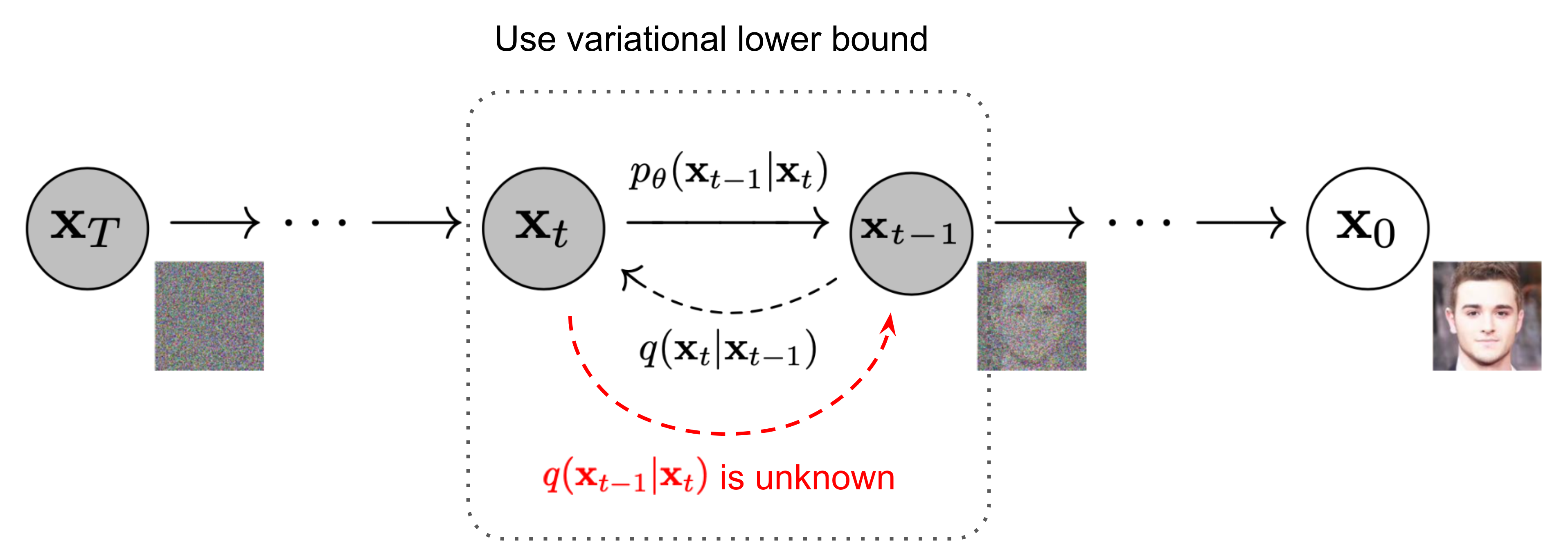
The Markov chain of forward (reverse) diffusion process of generating a sample by slowly adding (removing) noise.

we can let a image smaple(from real data distribution) $\mathbf{x}_0 \sim q(\mathbf{x})$

Usually we will also define steps $T$, where step size is controlled by ${\beta_t \in (0, 1)}_{t=1}^T$

With steps $T$, we can produce a sequence of noisy samples $x_1, x_2, …, x_T = z$

However, it is difficult to rebuild the image from $x_t$ to $x_0$ directly, we need the model to learn the rebuilt process piece by piece. i.e.

\[x_T \rightarrow x_{T-1} = u(x_T) \rightarrow x_{T-2} = u(x_{T-1}) \rightarrow ... \rightarrow x_1 = u(x_2) \rightarrow x_0 = u(x_1)\]

Destruction (Forward Process)

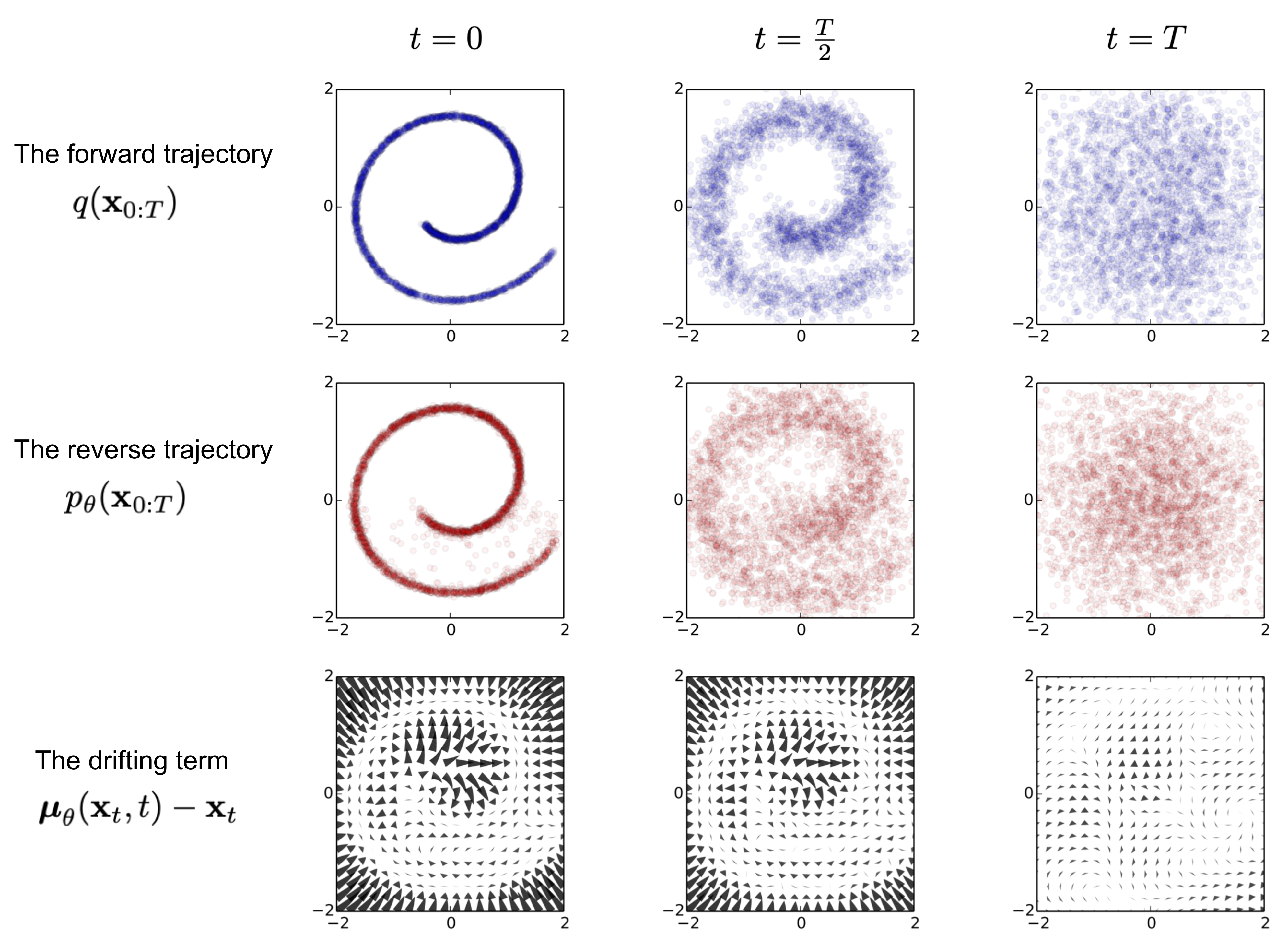
I’d like to use destruction instead of forward process. Basically we want to make a image (with pattern) to a pure gaussian noise by putting more gaussian noise recursively (with a fixed number of steps).

Sum of two Gaussian distribution

Two Gaussian ,e.g. $\mathbb{N}(0,\sigma^2_1 \boldsymbol{I}) \And \mathbb{N}(0,\sigma^2_2 \boldsymbol{I})$ with different variance can be merged to $\mathbb{N}(0,(\sigma^2_1+\sigma^2_2) \boldsymbol{I})$

By Wiki, Let $X$ and $Y$ be independent random variables that are normally distributed (and therefore also jointly so), then their sum is also noramlly distributed, i.e., if
\[\begin{aligned} X &\sim \mathbb{N}(\mu_X, \sigma^2_X) \\ X &\sim \mathbb{N}(\mu_Y, \sigma^2_Y) \\ Z &= X+Y \\ \end{aligned}\]
then
\[Z \sim \mathbb{N}(\mu_X+\mu_Y, \sigma^2_X+\sigma^2_Y)\]

Proof

Recall the theorem of variance.

\[\mathbb{V}(X+Y) = \mathbb{V}(X) + \mathbb{V}(Y) + 2\mathbb{Cov}(XY)\]

More generally, for random variables$X_1, X_2, \dots, X_N$, we have

\[\mathbb{V}\left(\sum_{i=1}^N a_i X_i\right)=\sum_{i=1}^N a_i^2 \mathbb{V}\left(X_i\right)+2 \sum_{i=1}^{N-1} \sum_{j=i+1}^N a_i a_j \operatorname{Cov}\left(X_i, X_j\right)\]

As $X_i \sim \mathbb{N}(\mu_i, \Sigma_i), i=1 \cdots N,$, we have claim they are i.i.d. Hence the covariances are zero. i.e. $\textbf{Cov}(X_i,X_j)=0$

A newly aggregated these Gaussian distributions is defined as a weighted sum:

\[X=\sum_{i=1}^{N} a_i X_i=\sum_{i=1}^{N} \frac{n_i}{\sum_{l=1}^{N}n_l} X_i, \\ \text{where} \sum_{i=1}^N a_i = 1\]

Therefore, we can find the merged variance as:

\[\begin{aligned} \text{Consider } \mathbb{X}_i &\sim \mathbb{N}(\mu_i, \Sigma_i) \\ \mu &= \sum_{i=1}^{N} a_i \mu_i \\ \Sigma &=\mathbb{V}(X)= \mathbb{V}(\sum_{i=1}^{N} a_i X_i)\\ &=\sum_{i=1}^{N}a_i^2\mathbb{V}(X_i) + 2 \sum_{i=1}^{N-1}\sum_{j=i+1}^{N} a_i a_j \textbf{Cov}(X_i,X_j) \\ & = \sum_{i=1}^{N}a_i^2 \Sigma_i + 0 \\ & = \sum_{i=1}^{N}a_i^2 \Sigma_i \end{aligned}\]

Details on destruction process

we define each step as

\[\boldsymbol{x}_t = \sqrt{\alpha_t}\boldsymbol{x}_{t-1} + \sqrt{\beta_t}\epsilon_t , \epsilon_t \sim \boldsymbol{N}(0, \boldsymbol{I}), \text{ where } \alpha_t + \beta_t = 1 \text{ and } \beta \approx 0\]

and let

\[\bar{\alpha}_t = \prod^t_{i=1}\alpha_i\]

, we have

\[\begin{aligned} \mathbf{x}_t &= \sqrt{\alpha_t}\mathbf{x}_{t-1} + \sqrt{1 - \alpha_t}\boldsymbol{\epsilon}_{t-1} \space \text{ ;where } \boldsymbol{\epsilon}_{t-1}, \boldsymbol{\epsilon}_{t-2}, \dots \sim \mathcal{N}(\mathbf{0}, \mathbf{I}) \\ \frac{\mathbf{x}_t}{\sqrt{\alpha_1\dots\alpha_t}} - \frac{\mathbf{x}_{t-1}}{\sqrt{\alpha_1\dots\alpha_t}} &= \frac{\sqrt{1-\alpha_t} \boldsymbol{\epsilon}_{t-1}}{\sqrt{\alpha_1\dots\alpha_t}} \\ \frac{\mathbf{x}_T}{\sqrt{\alpha_1\dots\alpha_T}} - \mathbf{x}_0 &= \sum^T_{t=1} \frac{\sqrt{1-\alpha_t} \boldsymbol{\epsilon}_{t-1}}{\sqrt{\alpha_1\dots\alpha_t}} \\ \mathbf{x}_T &= \sqrt{\alpha_1\dots\alpha_T}\mathbf{x}_0 + \sqrt{\alpha_{t+1}\dots\alpha_T}\sqrt{1-\alpha_t}\boldsymbol{\epsilon}_{t-1}\\ &= \sqrt{(a_t\dots a_1)} \mathbf{x}_0 + \sqrt{1 - (a_t\dots a_1)}\boldsymbol{\bar{\epsilon}}\\ &= \sqrt{\bar{\alpha}_t}\mathbf{x}_0 + \sqrt{1 - \bar{\alpha}_t}\boldsymbol{\bar{\epsilon}} \\ q(\mathbf{x}_t \vert \mathbf{x}_0) &= \mathcal{N}(\mathbf{x}_t; \sqrt{\bar{\alpha}_t} \mathbf{x}_0, (1 - \bar{\alpha}_t)\mathbf{I}) \end{aligned}\]

where $\boldsymbol{\bar{\epsilon}}$ is a sum of i.i.d gaussian noise

Therefore, we can observe by more steps iterated, the more image will be converted to pure noise.

Schedule

The formula

\[\bar{\alpha}_t = \prod^t_{i=1}\alpha_i\]

is formed by a schedule. The schedule is responsible to how the way is to destruct an image to pure noise.

Linear Schedule

The DDPM adopt linear schedule as follows:

def linear_beta_schedule(timesteps):
    beta_start = 0.0001
    beta_end = 0.02
    return torch.linspace(beta_start, beta_end, timesteps)

linear schedule

Cosine Schedule

Later cosine schedule is proponsed. It replace the linear schedule as:

In linear schedule, the last couple of timesteps already seems like complete noise
and might be redundan.
Therefore, Information is destroyed too fast.

Cosine schedule can solve the problem mentioned above.

Connection with frequency and destruction

Illustration of forward process

At small t, most of the low frequency contents are not perturbed by the noise, but high frequency content are being perturbed.
At bigger t, low frequency contents are also perturbed.
At the end of forward process, we get rid of the both low and high frequency contents of image.

Building (Reverse Process)

圖 3

We know how to process the forward process. However we have no idea to recover an image from noise as we dont know the formula, or equation for it. Luckily we can use deep neural network to approximate one due to Universal Approximation Theorem.

However, it is mentioned that it is difficult to recover/ generate directly from

\[x_t \rightarrow x_0\]

. Therefore, the intuitive idea is to find

\[q(x_{t-1}\vert x_t)\]

repeatedly and remove the noise (denoise) the image piece by piece. i.e.

\[\begin{aligned} \boldsymbol{x}_{t-1} &= \frac{1}{\sqrt{\alpha_t}}(\boldsymbol{x}_t - \sqrt{\beta_t}\epsilon_t) \\ \therefore \boldsymbol{\mu}(\boldsymbol{x}_t) &= \frac{1}{\sqrt{\alpha_t}}\left(\boldsymbol{x}_t - \sqrt{\beta_t} \boldsymbol{\epsilon}_{\boldsymbol{\theta}}(\boldsymbol{x}_t, t)\right) \end{aligned}\]

where $\theta$ is trainable parameters

Therefore, we can focus on and formulate a loss function by minimising predicted output $u(x_t)$ and groundtruth $x_{t-1}$ as

\[\begin{aligned} \mathbb{L} &= \left\Vert\boldsymbol{x}_{t-1} - \boldsymbol{\mu}(\boldsymbol{x}_t)\right\Vert^2 \\ &= \left\Vert\frac{1}{\sqrt{\alpha_t}}(\boldsymbol{x}_t - \sqrt{\beta_t}\epsilon_t) - \boldsymbol{\mu}(\boldsymbol{x}_t)\right\Vert^2 \\ &= \frac{\beta_t}{\alpha_t}\left\Vert \boldsymbol{\varepsilon}_t - \boldsymbol{\epsilon}_{\boldsymbol{\theta}}(\boldsymbol{x}_t, t)\right\Vert^2 \\ &= \frac{\beta_t}{\alpha_t}\left\Vert \boldsymbol{\varepsilon}_t - \boldsymbol{\epsilon}_{\boldsymbol{\theta}}(\sqrt{\bar{\alpha}_t}\mathbf{x}_0 + \sqrt{\bar{\beta}}\boldsymbol{\bar{\epsilon}}, t)\right\Vert^2 \end{aligned}\]

which is similar to loss function in DDPM (Ho et al., 2020)

\[\mathbb{E}_{\mathbf{x}_0, \boldsymbol{\epsilon}}\left[\frac{\beta_t^2}{2 \sigma_t^2 \alpha_t\left(1-\bar{\alpha}_t\right)}\left\|\boldsymbol{\epsilon}-\boldsymbol{\epsilon}_\theta\left(\sqrt{\bar{\alpha}_t} \mathbf{x}_0+\sqrt{1-\bar{\alpha}_t} \boldsymbol{\epsilon}, t\right)\right\|^2\right]\]

Therefore, we can train an network by minisming the captioned loss function, and generate a random image starting by $x_T \sim \boldsymbol{N}(0, \boldsymbol{I})$ to $x_0$ via

\[\boldsymbol{\mu}(\boldsymbol{x}_t) = x_{t-1} = \frac{1}{\sqrt{\alpha_t}}\big(\boldsymbol{x}_t - \sqrt{\beta_t} \boldsymbol{\epsilon}_{\boldsymbol{\theta}}(\boldsymbol{x}_t, t)\big)\]

which is simply an expression of

\[x_{t-1} \approx x_t - noise, \text{where } noise \sim \boldsymbol{N}(0,I)\]

in each step.

Summary

The training algorithm is 圖 1

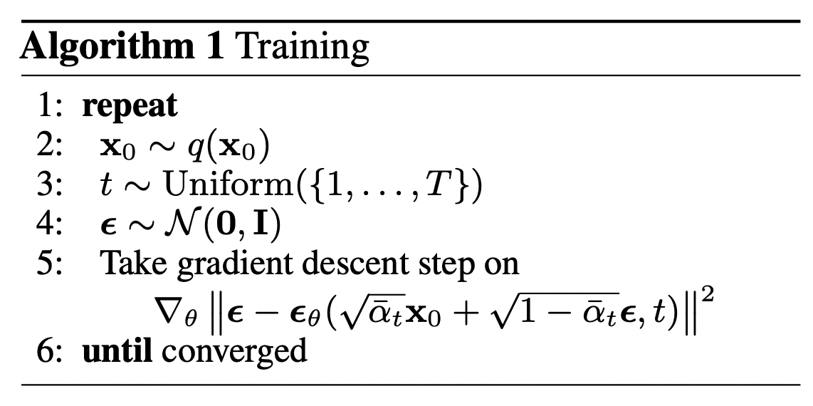
In other words:

we take a random sample $\mathbf{x}_0$ from the real unknown and possibily complex data distribution $q(\mathbf{x}_0)$
we sample a noise level $t$ uniformally between $1$ and $T$ (i.e., a random time step)
we sample some noise from a Gaussian distribution and corrupt the input by this noise at level $t$ (using the nice property defined above)
the neural network is trained to predict this noise based on the corrupted image $\mathbf{x}_t$ (i.e. noise applied on $\mathbf{x}_0$ based on known schedule $\beta_t$)

In reality, all of this is done on batches of data, as one uses stochastic gradient descent to optimize neural networks.

Review: Denoising Diffusion Probabilistic Models (DDPM)