Latent diffusion model (LDM)

Latent diffusion model(LDM) (Rombach & Blattmann, et al. 2022) runs the diffusion process in the latent space instead of pixel space, making training cost lower and inference speed faster.

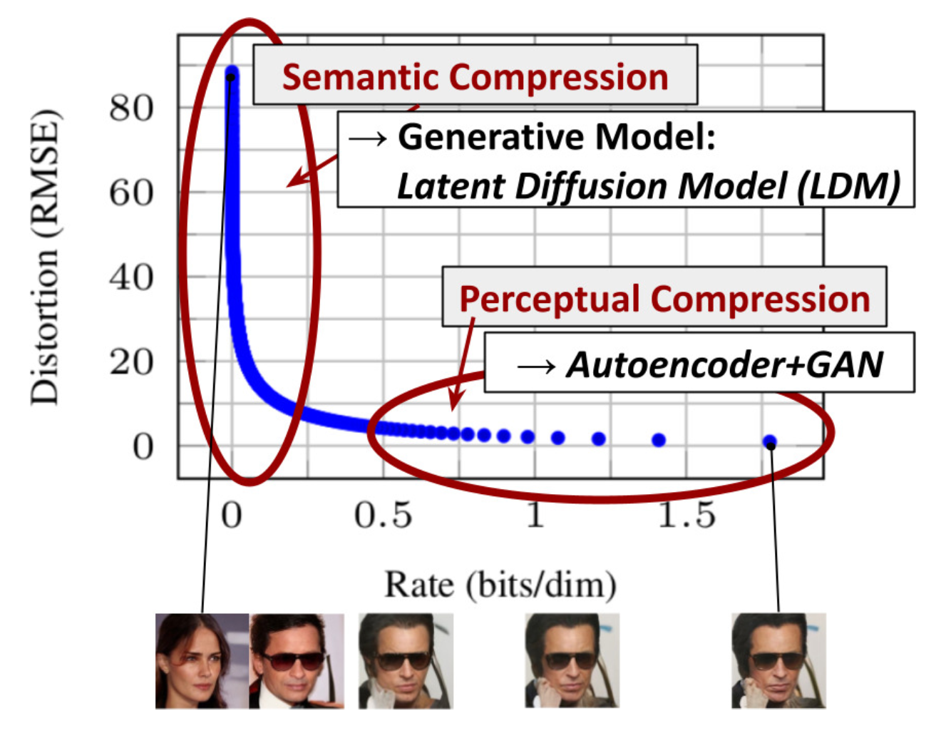
It is motivated by the observation that most bits of an image contribute to perceptual details and the semantic and conceptual composition still remains after aggressive compression. LDM loosely decomposes the perceptual compression and semantic compression with generative modeling learning by first trimming off pixel-level redundancy with autoencoder and then manipulate/generate semantic concepts with diffusion process on learned latent.

Latent representation from VAE

The perceptual compression process relies on an autoencoder model. An encoder $\mathcal{E}$ is used to compress the input image $x \in \mathbb{R}^{H\times W \times 3}$ to a smaller 2D latent vector $z = \mathcal{E}(x) \in \mathbb{R}^{h\times w \times c}$, where downsampling rate $f=H/h = W/w = 2^m, m \in \mathbb{N}$.

Then an decoder $\mathcal{D}$ reconstructs the images from the latent vector $\tilde{x} = \mathcal{D}(z)$.

Here the paper explored two types of regularization.

KL-reg: A small KL penalty towards a standard normal distribution over the learned latent, similar to VAE.
VQ-reg: Uses a vector quantization layer within the decoder, like VQVAE but the quantization layer is absorbed by the decoder.

Diffusion in Latent Space

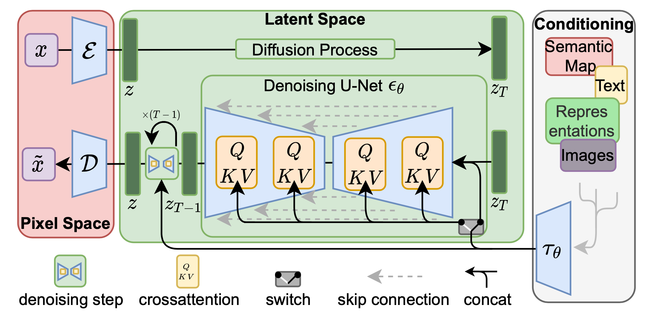The diffusion and denoising processes happen on the latent vector $z$. The denoising model is a time-conditioned U-Net, augmented with the cross-attention mechanism to handle flexible conditioning information for image generation (e.g. class labels, semantic maps, blurred variants of an image).

The design is equivalent to fuse representation of different modality into the model with cross-attention mechanism.

Each type of conditioning information is paired with a domain-specific encoder $\tau_\theta$ to project the conditioning input $y$ to an intermediate representation that can be mapped into cross-attention component.

Conditioned Generation

While training generative models on images with conditioning information such as ImageNet dataset, it is common to generate samples conditioned on class labels or a piece of descriptive text.

Classifier Guided Diffusion

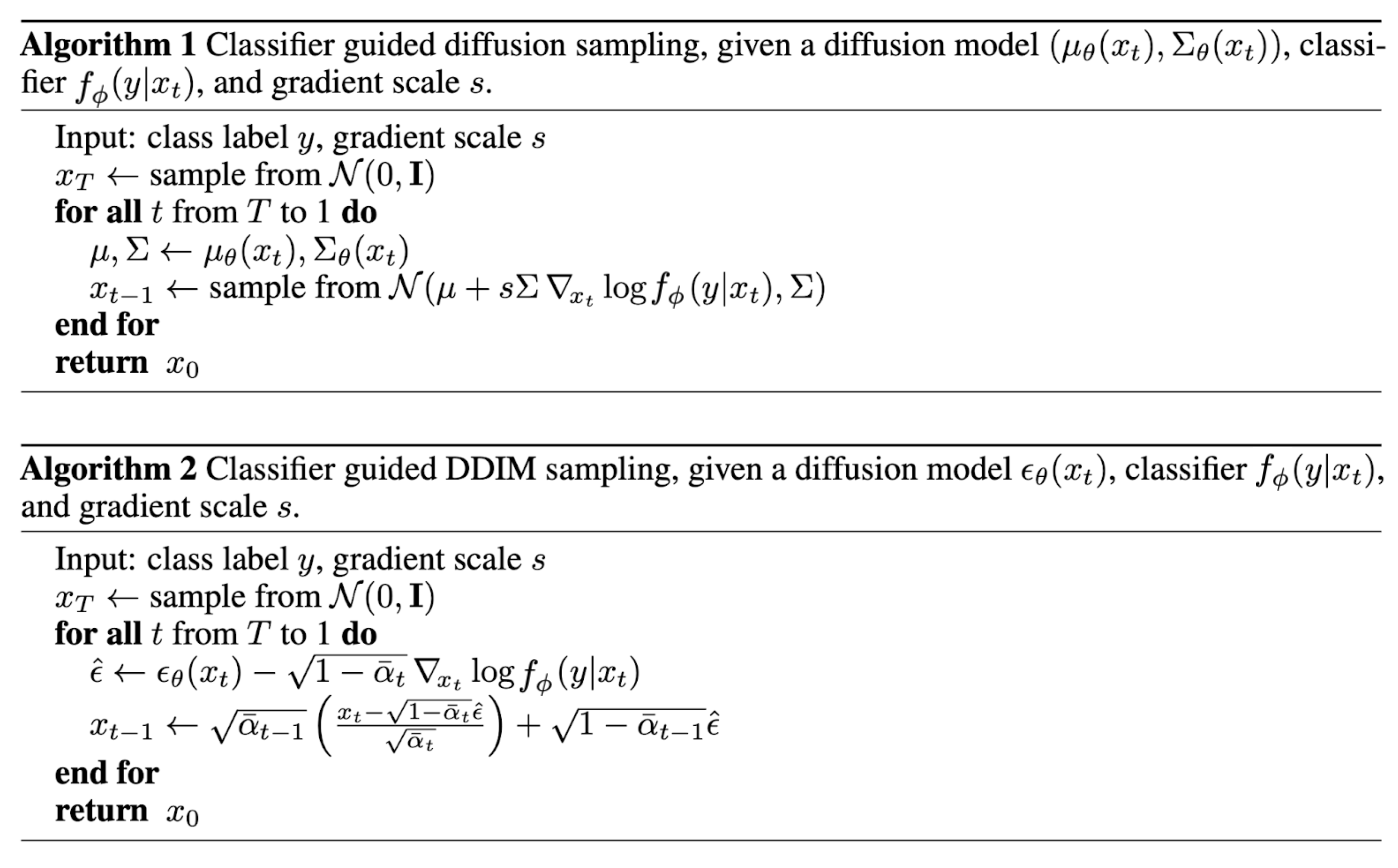
To explicit incorporate class information into the diffusion process, Dhariwal & Nichol (2021) trained a classifier $f_\phi(y\vert x_t,t)$ on noisy image $x_t$ and use gradients $\nabla_x log f_\phi (y\vert x_t)$ to guide the diffusion sampling process toward the conditioning information $y$ (e.g. a target class label) by altering the noise prediction.

Recall

\[\mu(x_t,t) = \frac{1}{\sqrt{\alpha_t}} \Big( x_t - \frac{1-\alpha_t}{\sqrt{1-\bar{\alpha}_t}}\epsilon_\theta(x_t,t) \Big)\]

Authors indicate that the following equation can be used to replace $\epsilon_\theta(x_t,t)$ to provide conditioning.

\[\tilde{\epsilon}(x_t) := \epsilon_\theta(x_t) - \sqrt{1-\bar{\alpha}_t} \nabla_{x_t} log f_\phi (y\vert x_t)\]

Proof

Langevin dynamics

Langevin dynamics is a concept from physics, developed for statistically modeling molecular systems. Combined with stochastic gradient descent, stochastic gradient Langevin dynamics (Welling & Teh, 2011) can produce samples from a probability density $p(\mathbf{x})$ using only the gradients $\nabla_\mathbf{x} \log p(\mathbf{x})$ in a Markov chain of updates:

\[\mathbf{x}_t = \mathbf{x}_{t-1} + \frac{\delta}{2} \nabla_\mathbf{x} \log q(\mathbf{x}_{t-1}) + \sqrt{\delta} \boldsymbol{\epsilon}_t ,\quad\text{where } \boldsymbol{\epsilon}_t \sim \mathcal{N}(\mathbf{0}, \mathbf{I})\]

where $\delta$ is the step size. When $T \rightarrow\infty, \epsilon \rightarrow 0, \mathbf{x}_T$ equals to the true probability density $p(\mathbf{x})$ .

Langevin dynamics in Diffusion Model

Song & Ermon, 2019 proposed a score-based generative modeling method where samples are produced via Langevin dynamics using gradients of the data distribution estimated with score matching. The score of each sample’s density probability is defined as its gradient $\nabla_{\mathbf{x}} \log q(\mathbf{x})$ A score network $s_\theta$ is trained to estimate it, s.t. $\mathbf{s}_\theta(\mathbf{x}) \approx \nabla_{\mathbf{x}} \log q(\mathbf{x})$

Given $\mathbf{x} \sim \mathcal{N}(\mathbf{\mu}, \sigma^2 \mathbf{I})$, we can write the derivative of the logarithm of its density function as

\[\nabla_{\mathbf{x}}\log p(\mathbf{x}) = \nabla_{\mathbf{x}} \Big(-\frac{1}{2\sigma^2}(\mathbf{x} - \boldsymbol{\mu})^2 \Big) = - \frac{\mathbf{x} - \boldsymbol{\mu}}{\sigma^2} = - \frac{\boldsymbol{\epsilon}}{\sigma}, \text{ where } \boldsymbol{\epsilon} \sim \mathcal{N}(\boldsymbol{0}, \mathbf{I})\]

Recall $q(\mathbf{x}_t \vert \mathbf{x}_0) \sim \mathcal{N}(\sqrt{\bar{\alpha}_t} \mathbf{x}_0, (1 - \bar{\alpha}_t)\mathbf{I})$

Therefore,

\[\mathbf{s}_\theta(\mathbf{x}_t, t) \approx \nabla_{\mathbf{x}_t} \log q(\mathbf{x}_t) = \mathbb{E}_{q(\mathbf{x}_0)} [\nabla_{\mathbf{x}_t} q(\mathbf{x}_t \vert \mathbf{x}_0)] = \mathbb{E}_{q(\mathbf{x}_0)} \Big[ - \frac{\boldsymbol{\epsilon}_\theta(\mathbf{x}_t, t)}{\sqrt{1 - \bar{\alpha}_t}} \Big] = - \frac{\boldsymbol{\epsilon}_\theta(\mathbf{x}_t, t)}{\sqrt{1 - \bar{\alpha}_t}}\]

In short,

\[\nabla_{\mathbf{x}_t} \log q(\mathbf{x}_t) = - \frac{1}{\sqrt{1 - \bar{\alpha}_t}} \boldsymbol{\epsilon}_\theta(\mathbf{x}_t, t)\]

Therefore we can write the score function for the joint distribution $q(x_t, y)$ as following,

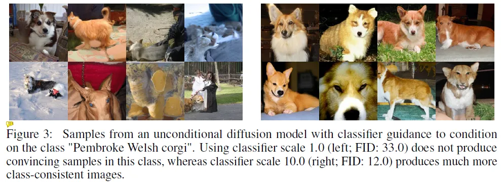
\[\begin{aligned} \nabla_{\mathbf{x}_t} \log q(\mathbf{x}_t, y) &= \nabla_{\mathbf{x}_t} \log q(\mathbf{x}_t) + \nabla_{\mathbf{x}_t} \log q(y \vert \mathbf{x}_t) \\ &\approx - \frac{1}{\sqrt{1 - \bar{\alpha}_t}} \boldsymbol{\epsilon}_\theta(\mathbf{x}_t, t) + \nabla_{\mathbf{x}_t} \log f_\phi(y \vert \mathbf{x}_t) \\ &= - \frac{1}{\sqrt{1 - \bar{\alpha}_t}} (\boldsymbol{\epsilon}_\theta(\mathbf{x}_t, t) - \sqrt{1 - \bar{\alpha}_t} \nabla_{\mathbf{x}_t} \log f_\phi(y \vert \mathbf{x}_t)) \end{aligned}\]

Lastly, one extra hyper-parameter gradient scale is introduced to form the samplng equation. 圖 3

Result is improved due to guided classifer 圖 1

Classifier-Free Guidance

Without an independent classifier $p_\phi$, it is still possible to run conditional diffusion steps by incorporating the scores from a conditional and an unconditional diffusion model (Ho & Salimans, 2021). Let unconditional denoising diffusion model $p_\theta(\mathbf{x})$ parameterized through a score estimator $\boldsymbol{\epsilon}_\theta(\mathbf{x}_t, t)$ and the conditional model $p_\theta (x\vert y)$ parameterized through $\boldsymbol{\epsilon}_\theta(\mathbf{x}_t, t, y)$ . These two models can be learned via a single neural network. Precisely, a conditional diffusion model $p_\theta(\mathbf{x} \vert y)$ is trained on paired data $(x,y)$ , where the conditioning information $y$ gets discarded periodically at random such that the model knows how to generate images unconditionally as well, i.e. $\boldsymbol{\epsilon}_\theta(\mathbf{x}_t, t) = \boldsymbol{\epsilon}_\theta(\mathbf{x}_t, t, y=\varnothing)$ .

The gradient of an implicit classifier can be represented with conditional and unconditional score estimators. Once plugged into the classifier-guided modified score, the score contains no dependency on a separate classifier.

\[\begin{aligned} \nabla_{\mathbf{x}_t} \log p(y \vert \mathbf{x}_t) &= \nabla_{\mathbf{x}_t} \log p(\mathbf{x}_t \vert y) - \nabla_{\mathbf{x}_t} \log p(\mathbf{x}_t) \\ &= - \frac{1}{\sqrt{1 - \bar{\alpha}_t}}\Big( \boldsymbol{\epsilon}_\theta(\mathbf{x}_t, t, y) - \boldsymbol{\epsilon}_\theta(\mathbf{x}_t, t) \Big) \\ \bar{\boldsymbol{\epsilon}}_\theta(\mathbf{x}_t, t, y) &= \boldsymbol{\epsilon}_\theta(\mathbf{x}_t, t, y) - \sqrt{1 - \bar{\alpha}_t} \; w \nabla_{\mathbf{x}_t} \log p(y \vert \mathbf{x}_t) \\ &= \boldsymbol{\epsilon}_\theta(\mathbf{x}_t, t, y) + w \big(\boldsymbol{\epsilon}_\theta(\mathbf{x}_t, t, y) - \boldsymbol{\epsilon}_\theta(\mathbf{x}_t, t) \big) \\ &= (w+1) \boldsymbol{\epsilon}_\theta(\mathbf{x}_t, t, y) - w \boldsymbol{\epsilon}_\theta(\mathbf{x}_t, t) \end{aligned}\]

In short, we can add an additional condition to model s.t. $\epsilon_\theta(x_t) \rightarrow \epsilon_\theta(x_t,y)$. This method can combine both condition and unconditional cases st. $\epsilon_\theta(x_t,y) \And \epsilon_\theta(x_t,y=Null)$ . In reserve process, we can use

$\tilde{\epsilon}_\theta(x_t \vert y) = \epsilon_\theta (x_t) + s\cdot(\epsilon_\theta(x_t,y) - \epsilon_\theta(x_t))$ , where s is a strengh hyperparameter.

Review: High-Resolution Image Synthesis with Latent Diffusion Models (LDM)